Linear regression: Similarities and differences between homoscedasticity test of plain and Student residuals?

[DynV]

About the following translation on linear regression: What are the similarities and differences between homoscedasticity test of plain and Student residuals? Are they just 2 ways of doing the same technique of linear regression assumption verification, or are they 2 different techniques? If they're different, is there similarities in between, and if so which? The code is in R. There's text after the image. What's below is a translation of the lesson.

We can check the homogeneity of variances and normality using the same tools as for ANOVA.

by(mfrow = c(1, 2), cex = 1.2)
##homogeneity of variance
plot(residuals(m1) ~ fitted(m1), ylab = "Residuals",
xlab = "Predicted values",
main = "Homogeneity of variances")
##normality
text("a", x= 2.3, y = 0.7, cex = 1.2)
qqnorm(residuals(m1), ylab = “Observed quantiles”,
xlab = "Theoretical quantiles",
main = "Normality of residues")
qqline(residuals(m1))
text("b", x= -1.4, y = 0.7, cex = 1.2)

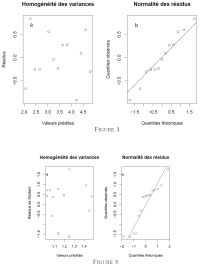
Figure 3a shows that the variances are homogeneous. Although some residuals deviate from normality (3b), linear regression is appropriate.

##checks assumptions
by(mfrow = c(1, 2), cex = 1.2)
plot(rstudent(m.shocks) ~ fitted(m.shocks),
ylab = “Student Residuals”,
xlab = "Predicted values",
main = "Homogeneity of variances")
text(y = 1.5, x = 1.025, labels = "a")
qqnorm(rstudent(m.shocks), ylab = “Observed quantiles”,
xlab = "Theoretical quantiles",
main = "Normality of residues")
qqline(rstudent(m.shocks))
text(y = 1.5, x = -1.9, labels = "b")

The diagnostic plots show that the variances are approximately homogeneous and that the residuals approximately follow a normal distribution (Fig. 8). Since we used Student residuals, we were able to confirm at the same time the absence of extreme values in fig. 8a).

 

[BigBeachBanana]

What are the similarities and differences between homoscedasticity test of plain and Student residuals? Are they just 2 ways of doing the same technique of linear regression assumption verification, or are they 2 different techniques? If they're different, is there similarities in between, and if so which?

They differ in how the residuals are computed.
For the "plain", [imath]e_i=y_i-\hat{y}_i[/imath], observed minus prediction.
Whereas the student's residual is [imath]t_i=\dfrac{e_i}{\hat{\sigma}(e_i)}[/imath], where [imath]\hat{\sigma}[/imath] is the estimate of the standard deviation of the i-th residual.

The "plain" residual is straightforward to compute. On the other hand, the student's residual is more robust but expensive to compute.

 

[DynV]

I mean, is there some direct link between the 2 as in you invert something from the other, make a quadratic function or whichever method? eg method2 = functionX(method1) - functionY(method1) ?

 

[BigBeachBanana]

is there some direct link between the 2

The students use the [imath]e_i[/imath].

as in you invert something from the other, make a quadratic function or whichever method? eg method2 = functionX(method1) - functionY(method1) ?

I don't understand the rest of what you're asking here.

 

[Otis]

is there some direct link between the 2 as in you invert something from the other

Hi. If you're asking whether e_i and t_i have an inverse relationship, then the answer is no. To me, it looks like t_i is a scaled version of e_i.

The verb 'invert' means something else. For example, inverting the ratio a/b yields its reciprocal b/a.
[imath]\;[/imath]

 

[DynV]

I don't understand the rest of what you're asking here.

Hi. If you're asking whether e_i and t_i have an inverse relationship, then the answer is no.

"as in you [...] or whichever method" they were examples.